Analyze one dependent variable and produce everything a paper needs

One-call pipeline for a single dependent variable: checks the assumptions (producing a ready-made methods sentence via assumption_methods_text()), builds the matching ggstatsplot figure with automatic parametric/non-parametric selection, reports the omnibus test via reportggstatsplot(), and – for more than two groups – reports the significant post-hoc comparisons via reportggstatsplotPostHoc().

Usage

analyze_and_report(
  data,
  dv,
  iv,
  design = c("between", "within"),
  ylab = dv,
  xlabels = NULL,
  plotType = "boxviolin",
  sink_to = NULL
)

Arguments

data

the data frame

dv

the dependent variable (column name as string)

iv

the independent variable (column name as string); coerced to a factor if it is not one already

design

"between" for between-subjects data (default) or "within" for repeated measures

ylab

label for the dependent variable; defaults to dv

xlabels

optional labels for the x-axis

plotType

either "box", "violin", or "boxviolin" (default)

sink_to

optional path of a .tex file; the methods sentence, omnibus result, and post-hoc sentences are written there so a manuscript can \input{} them

Value

Invisibly returns a list with components plot (the ggplot), methods (assumption-check sentence), text (omnibus result), posthoc (post-hoc sentences, or NULL for two groups), and sentences (all text combined, in manuscript order).

Examples

# \donttest{
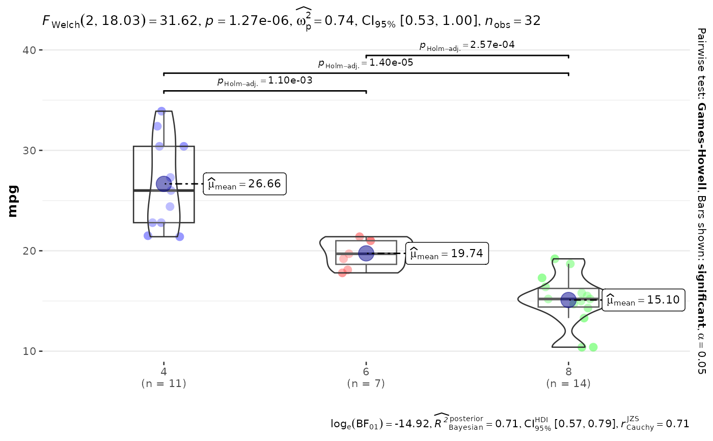
result <- analyze_and_report(mtcars, dv = "mpg", iv = "cyl")
#> Shapiro--Wilk tests indicated no significant deviation from normality in any group (all $p \geq 0.05$); therefore, parametric tests were used. Levene's test indicated unequal variances ($F(2, 29) = 5.51$, $p = 0.009$); Welch-corrected statistics were used where applicable.
#> An One-way analysis of means (not assuming equal variances) found a significant effect of \cyl on mpg (\F{2}{18.03}{31.62}, \pminor{0.001}, r=0.74). 
#> A Games-Howell post-hoc test found that 4 was significantly higher (\m{26.66}, \sd{4.51}) in terms of \mpg compared to 6 (\m{19.74}, \sd{1.45}; \padj{0.001}). 
#> A Games-Howell post-hoc test found that 4 was significantly higher (\m{26.66}, \sd{4.51}) in terms of \mpg compared to 8 (\m{15.10}, \sd{2.56}; \padjminor{0.001}). 
#> A Games-Howell post-hoc test found that 6 was significantly higher (\m{19.74}, \sd{1.45}) in terms of \mpg compared to 8 (\m{15.10}, \sd{2.56}; \padjminor{0.001}). 
result$plot

# }